Classification: y = 0 or y = 1
if hθ(x) ≥ 0.5, predict y=1
if hθ(x) < 0.5, predict y=0
⇒ logistic regression: 0 ≤ hθ(x) ≤ 1
Hypothesis Representation
- Sigmoid function (==logistic function)

(cf) hθ(x) = 0.7 ⇒ 70% chance of ~~~
Decision boundary
hθ(x) = g(θ0+θ1x1+θ2x2) ⇒ predict y=1 if -3+x1+x2 ≥ 0
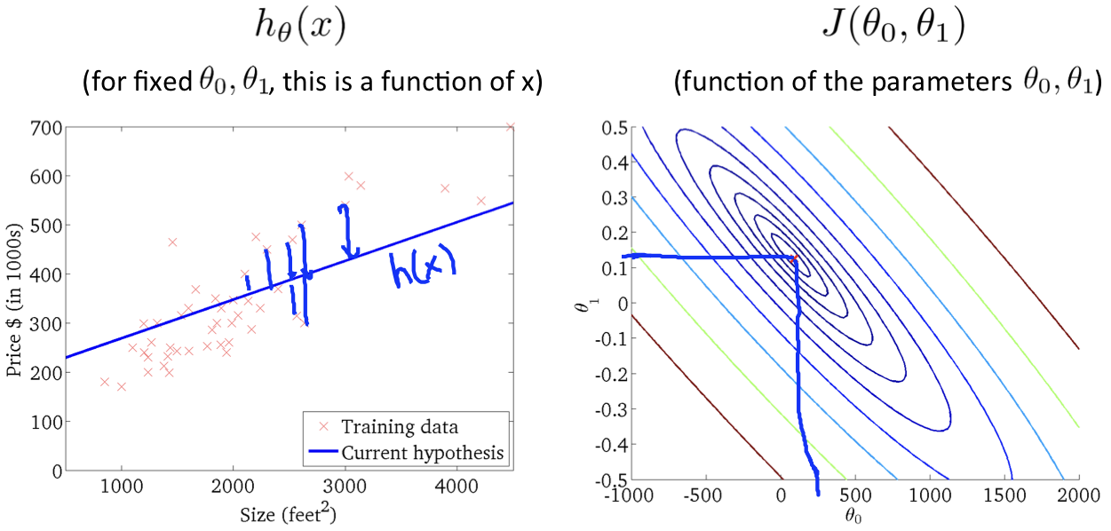
Cost function
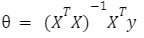
- How to choose parameter θ?
Simplified cost function and gradient descent
* convert the two lines into one line
Logistic regression cost function
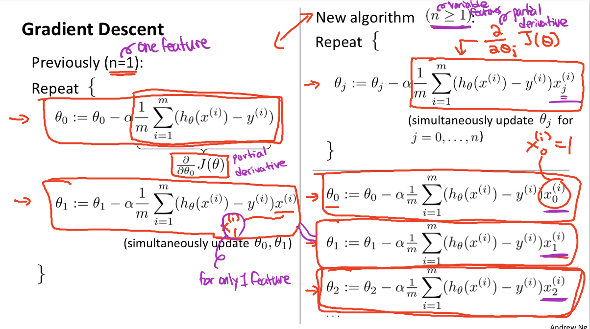
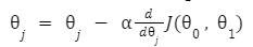
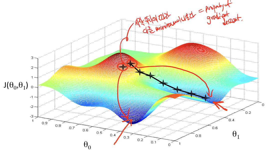
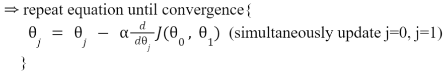
Gradient Descent
*Looks same as linear regression!
BUT, hθ(x) are different! ==>
![]()
Multi-class classification (one-vs-all)
Sigmoid function VS softmax classifier
⇒ sigmoid: get percentage on how y might equal to 1 for each class
⇒ softmax: get the distribution of percentage of the classes
'AI NLP Study > Machine Learning_Andrew Ng' 카테고리의 다른 글
| Coursera - Machine Learning_Andrew Ng - Week 2 (0) | 2022.01.25 |
|---|---|
| Coursera - Machine Learning_Andrew Ng - Week 1 (0) | 2022.01.25 |